Regularization

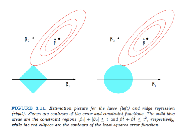
In the previous article, when we were talking about feature selection, we mentioned that it may be difficult to determine ahead of time which features are important and which features are irrelevant. To solve this issue, many ML engineers use regularization. Instead of blindly picking and choosing features to use at the risk of losing important information, it is often useful to just use all features but regularize them as well. Thus, in implementation, regularization is applied as a safety measure by default and is applied to all features. Applying regularization by default also safeguards against getting an overfitted model even though we are using all features. To implement regularization, it is necessary to have a modified cost function. This looks different depending on what kind of regression it is.

Linear Regression with Regularization

cost = J(w, b) = 1/2m(∑^m_{i = 1}(f_w,b(x⁽ⁱ⁾) - y⁽ⁱ⁾))² + λ/2m((∑ⁿ_{j = 1}(w_j)²))

Lambda is called the regularization parameter. It is a constant that we must choose (similar to the learning rate alpha). If lambda is 0, the model will overfit. If lambda is a large number, the model will underfit.

Thus, we have added an additional term to the mean-squared error cost function. When doing gradient descent, it is necessary to also minimize this added term. Note that by convention, we tend not to regularize the b parameter.

Gradient Descent for Linear Regression with Regularization

Gradient descent will also look different due to this added regularization term. Notice that the updating of the b term remains the same because we do not need to regularize b.

The added regularization term serves to shrink the value of w a little bit with each iteration. Over time, the w terms get shrunk significantly and their weight is reduced.

Logistic Regression with Regularization

cost = J(w, b) = -1/m(∑^m_{i = 1}y⁽ⁱ⁾log(f_w,b(x)) + ((1-y)log(1- f_w,b(x)))) + λ/2m((∑ⁿ_{j = 1}(w_j)²))

By reducing the weights of each feature, regularization with logistic regression ensures that the decision boundary is not overfitted to the data.

Gradient Descient with Logistic Regression with Regularization

The cost function to minimize is already given above. To implement gradient descent,

This looks the same as the gradient descent formulas for linear regression with regularization; the only difference is that the definition of f_{w, b} is not wx + b but is now the sigmoid function g(z) where z = wx + b.